Joao Reis - FEUP

Zero-shot Learning

One of the most intriguing and fascinating capabilities of humans is to generalize upon multiple and diverse tasks. When only presented with few examples, humans can quickly learn particular features of a certain object or task, distinguishing it from different classes of objects. The human capability to generalize allows to extrapolate and infer which kind of physical object it might be from previously seen examples of different object classes. As presented by Biederman (1987), humans have the capability to identify and distinguish about 30,000 objects, and for each of these objects there was no need for showing a million images of the same object in order to recognize and discriminate it from other objects, as it is often required in deep learning approaches such as in convolutional neural networks (CNNs). In fact, a great majority of humans would become confused if such an amount of images of the same object was shown to them. Instead, based on a small amount of images, or even from an object description, humans can generalize by extracting certain features of an object and form high level representations. By relating all the information learned and internal object representations, it is easier to learn from small amount of pictures. This capability to extract particular features and properties of an object and then generalize to other unseen classes of objects is one of the greatest challenges in artificial intelligence nowadays.

A definition for this particular type of problem was first presented by Larochelle et al.(2008) where it first called zero-data learning and defines it as follows: "Zero-data learning corresponds to learning a problem for which no training data are available for some classes or tasks and only descriptions of these classes / tasks are given.". Humans can imagine and mentally visualize certain objects when reading a book or an article, or just by thinking about certain past stories. Based on 1) a description of the object and 2) prior knowledge about the world, humans can materialize such imagined objects by drawing, sculpturing or even 3D modeling and recognize these if seen somewhere else. This is the main idea to explore in zero-data learning, that was afterwards named as zero-shot learning. If this description about an object is available, based on all the learning throughout lifetime humans can match their own mental visualization of an object with the physical one, and determine if these are the same or somehow similar in certain features. Normally, in such situations, intuition plays a significant role by matching an already learned object, problem or pattern, and immediately recognizing it without great effort. Such concepts are the ones that ZSL is based on to build a set of algorithms and strategies for machine learning.

The main motivation behind ZSL is that, as depicted and explored by Larochelle et al. (2008), the number of tasks is far too large and data for each task is far too little. We have already seen some great advances in artificial intelligence where systems reach superhuman capabilities in very specific tasks. Despite all these great achievements, these are not even close to the generalization of human capability and knowledge transfer from a set of tasks to new unseen ones. ZSL can be one of the tools to achieve such generalization capability.

In practical terms, the main idea of ZSL is to correctly classify an image based on a set of already learned tasks and a description of these tasks and the new task to be learned. Thus, in this context, normally the classes used in the training process are different from the ones in the test procedure. In other words, the system should derive a solution for a particular unseen class from the introduced classes. For this case, the task descriptors play a significant role and is based on them that this "derivation" happens. In sum, once some input is presented together with its class / task descriptor, a classifier or predictor should provide the correct output for that specific problem.

Zero-Shot Learning for Regression

So far, we have seen ZSL approaches that try to solve the problem of classifying new instances from classes that were not used in the training process. This means that a trained algorithm tries to correctly label a new instance from a class without being trained to do so. One of the key aspects to achieve a good performance is to have an additional feature space (often called latent space) that describes each task, where normally a meta-description of each task is used, apart from input and output feature spaces. This is one property that inspired the development of the proposed approach.

Despite the good results achieved in the works presented in the previous section, non of them are neither designed nor applied to regression problems. Regression maps certain inputs into a set of continuous output variables, while in classification the output is either 0 or 1, or in a range between 0 and 1 such as in probabilistic models. Nevertheless, regression is used in these works to help, e.g. map the inputs into a continuous latent space such as the coefficients of a linear classifier, as presented in Larochelle et al. (2008). However, the application of the problem is never regression. Most of the works are related with classification problems ranging from image classification to molecular compound matching or object classification from haptic data. Here, we present an approach called hyper-process model (HPM) that addresses the problem of ZSL for regression problems.

Problem Definition

As a first step, we would like to define the problem of ZSL to regression. Up to our knowledge, this is the first work that makes such a definition for regression. Related with image classification, most of the ZSL techniques take advantage on the difference between input images, which is something normal where two different objects are displayed. Assuming inputs for a certain class / task as $X_i \in \mathcal{X}$ for class $i$ , we can say that these techniques assume $P(X_i) \neq P(X_j)$ where marginal distributions among classes are not the same. This means that the difference between the images can be learned to separate both from different classes. Contrary to this, for ZSL in regression problems the inputs for different tasks could be the same and the responses might be different according to their specific task. For example, the amount of traffic in different parts of the city can be the same $P(X_i) = P(X_j)$ , where $i$ and $j$ represent different parts of the city, but the air quality might be different because of different amounts of vegetation. If one part of the city has more vegetation, the air quality is higher, and vice versa. Most of the works first try to map the input into a latent space, which normally is a task descriptor, that can be generally expressed as $\mathcal{G} : X^n \rightarrow F^k$ , where $X \in \mathbb{R}^n$ are inputs and $F \in \mathbb{R}^k$ are the task descriptors. In order to successfully learn the differences between tasks or classes, there should exist some difference between the task inputs like cubes and spheres, or cats and houses. Therefore, the assumption of $P(X_i) \neq P(X_j)$ is implicit in the context of image classification, which might not hold true for regression. Hence, this draws the first difference between how ZSL works for classification and regression, where it is not assumed that the marginal distribution of inputs from different tasks are different, and hence the proposed technique is applicable for problems where $P(X_i) = P(X_j)$ .

Additionally, another key difference between ZSL for classification and regression is that multiple image classes are learned at the same time as a multi-task learning fashion. For the particular case of ZSL in classification, we have already previously seen that this learning normally occurs in two different steps: 1) Learning a mapping between inputs and task description, and 2) Task description into class labels. This means that only one classifier should learn the differences between images and correctly predict the corresponding task description, and also a classifier that handles the predicted task description should correctly classify it into the desired class labels. Ultimately, the final goal of ZSL in classification is to provide a new unseen image and correctly predict the label from a class not used in the learning process. Opposite to this idea, for the regression setting, the main goal is to build a whole new predictive function suitable for the new unseen task, where multiple inputs can be fed as a regular regressor. Therefore, for each source task, a regressor needs to be previously learned and together with the task description, a new function should be derived for a target task. The only work that uses the same approach is the already depicted technique called model space view presented by Larochelle et al. (2008). Additionally, the same principle was applied to solve a concrete problem in the area of manufacturing systems named hyper-model (HM) (Pollak and Link (2016)). Despite these techniques being in fact applicable for regression, the proposed approach overtakes some limitations of such techniques. These will be presented later in this section, and will be highlighted and explained with a theoretical example.

In sum, we can define the ZSL for regression problem in the context of this work as the generation of a predictor that can be used in a new, unseen task, based on 1) task descriptions for both source and target tasks and 2) a set of predictors, one for each source task. Hence, we should define a task description as $c_i \in C$ for task $i$ , where $C$ is defined as all the source task descriptions; and the predictors as $f_i \in F$ , where $F$ is defined as a set of functions. For the latter, we should define a function as $f_i : X \rightarrow Y$ , where $X$ and $Y$ are the input and output feature spaces, correspondingly. Additionally to all of this, we should also define a function that maps the task descriptions into a latent space $\mathcal{L} : C \rightarrow Z^p$ , where $Z$ is the latent space in a $p$ -dimensional space. If each of the predictors of the source tasks has a set of trained parameters $\theta$ and all the predictors have the same number of parameters, this approach would be identical to the one presented by Larochelle et al. (2008) where $Z^p$ represents the same as $\theta$ , so the parameters of the new function $\theta'$ would be predicted by $\mathcal{L}$ providing the target task description $c_t$ , being $t$ the target task. However, the key difference between the proposed approach and the one presented by Larochelle et al. (2008) is that the feature space $Z^p$ is not the a set of function coefficients. In the proposed approach the feature space is independent from the function coefficients and in fact do not assume that the number of coefficients should be same for all the functions used to learn the source tasks. For example, in order to learn a predictor that maps task descriptions into function coefficients, one should choose the type of machine learning technique to use, such as degree 2 polynomial, to train all the source tasks. In Larochelle et al. (2008) and Pollak and Link (2016), this implies that all source tasks will be trained using the same technique, not exploring the possibility of using the best machine learning technique for each source task. We interpret this as a limitation, where different tasks might have different complexities, and therefore certain types of functions might be more suitable to some tasks, and not to others. In the proposed approach we make use of a widely known technique from the computer vision area to address such a limitation, and create a common feature space for different machine learning techniques.

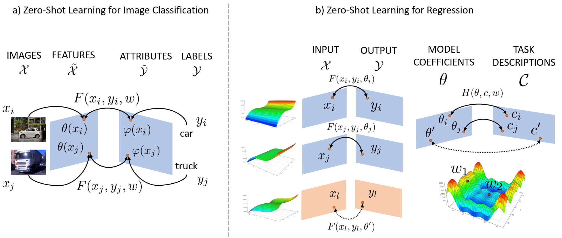
For a more complete explanation, Figure 1 makes a visual comparison between two approaches as a way to clearly make a distinction of ZSL for regression from ZSL for classification, in particular, to image classification. This way, on the left-hand side is a representation of the SJE approach (Akata et al., 2015) that makes use of two latent spaces, namely image embeddings and class embeddings. In this setting, the main idea is to present an unseen image from an unseen class during training, and correctly estimate its label. Contrary to this, the goal of ZSL for regression is to estimate a new model by making use of an unseen task description and previous knowledge about already existing models. Particularly for the hyper-model approach this learning is simply the mapping between coefficients and task descriptions of source models used to estimate the target model. This way, on the right-hand side two stages can be clearly seen. One is related with training the source models to derive the best models' coefficients $\theta$ for each task and the other is to train the hyper-model using those coefficients and existing task descriptions. Once a new task description is available, the model coefficients $\theta'$ can be estimated and a new function can be used $F(x_l,y_l,\theta')$ , where $x_l$ are the new input values that can be used to predict $y_l$ (orange boxes on the bottom represent the new generated function). Hence, this visual separation allows to clear draw the main differences between classification and regression settings for ZSL, where one tries to label unseen instances in a class not used during training, and the other tries to estimate a whole new function based on previous acquired knowledge of existing functions and task descriptions.

Figure 1: Comparison between ZSL for image classification and regression. a) Case where a latent representation for both images and classes is used, and a compatibility between these is learned (Akata et al., 2015). b) Case where multiple models are used to learn a hyper-model that maps model coefficients $\mathcal{\theta}$ into task descriptions $\mathcal{C}$ . Upon new task descriptions $c'$ , new model coefficients $\theta'$ can be estimated and a new model is created Pollak and Link (2016). This representation is also applicable in the model space view approach from Larochelle et al. (2008).

Hyper-Process Model (HPM)

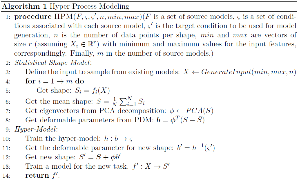
The main intentions of the present section is to, first, clearly present the full algorithm of hyper-process model (HPM) from the point of using the models trained with different techniques, to the final estimation of the new model to be used as a predictor in a new task. Secondly, it is intended to be reproducible for other researchers, where a step by step description of the algorithm is presented and explained. For that, most of the equations, notations and notions presented earlier are used, being the algorithm description just an organized way to present the approach.

Hence, Algorithm 1 presents all the steps required to implement the solution for different contexts of application. The first thing to notice is that the algorithm itself is divided into two different parts, as in the previous two subsections. This was intended so readers can easily relate to what was explained before and quickly find the content associated to each technique. Based on this, the algorithm starts to introduce all the parameters necessary for its execution. As described, all the trained models are required along with the corresponding conditions (which are the task descriptions from ZSL). Moreover, the target condition is required in order to generate the new model. Additionally, one should also specify the number of landmarks to use for each shape, together with two more vectors that define the minimum and maximum values for the input features space. These minimum and maximum vectors are required so one could generate the input values to sample from the trained models. Since we are assuming $P(X_s) = P(X_t)$ , only a vector is required and is used in all source tasks to generate shapes. Finally, we assume to have $m$ trained models to deal with.

For this algorithm, the SSM first comes into place because the hyper-model is dependent on the common representation of models to be trained. Hence, the first step (line 3) is to generate the input values $X$ according to the minimum, maximum and number of intended landmarks per shape. Since we assume that no information can be drawn between the different inputs from the various models (as stated by $P(X_i) = P(X_j)$ ), the same input values are used for all the models. Therefore, the shapes $S_i$ are built only considering the values from the output feature space, as presented in line 5, where $i$ is a specific model.

The next step is calculate the mean shape from all the generated shapes (line 6). In order to get all the eigenvectors to build the deformable model, a decomposition needs to be performed on all the generated shapes and PCA is applied (line 7). One should emphasize again that each shape is a vector of $kn$ elements, where $k$ is the number of features and $n$ is the number of landmarks to use. Therefore, PCA is performed on a $m \times kn$ matrix $S$ composed by all the shapes from source models, where these shapes are stacked in rows. Finally, the last step for the SSM is to derive all the deformable parameters for all the models (line 8). These are the parameters required to generate back the initial shape based solely on the deformable model. In order to get a good shape reconstruction the number of components chosen when performing PCA is critical, being a trade-off between reconstruction and complexity. On one hand, if few components are chosen, the greater the reconstruction error will be but less dimensions are required, and thus, less complex the problem is. On the other hand, if all the components are chosen, the reconstruction error will be minimum, but the complexity of the problem is far too great to deal with. In these situations, a good rule of thumb is to use the number of components (ordered by decreasing order of model variance) that attend for a cumulative sum of variance of at least 95%.

After building the deformable model, together with all the deformable parameters, the hyper-model is ready to be trained. For this case, and as presented by Pollak and Link (2016), one should train a hyper-model using any machine learning technique that seems suitable for the problem, by mapping deformable parameters into conditions. One might think at this stage that would be more suitable to map conditions into deformable parameters instead, because we can use the trained model to predict the parameters based on new conditions. However, in most of the cases the dimension of the deformable parameters are greater than conditions, so the modeling needs to be made according to line 10. Only in the cases where 1) the dimension of parameters is the same or lower than conditions or 2) multiple models are trained as a hyper-model and each one of those models has only an output variable different from the others, the model can be trained as follows $h : \varsigma \rightarrow b$ . The implication of building a hyper-model that maps deformable parameters into conditions is visible in line 11, where the technique used needs to be invertible in order to get the new deformable parameters according to the specified new conditions. As an alternative, the level set where the model surface intercepts with the hyper-plane for the intended target condition can be calculated, as performed in the work of Pollak et al. (2011), or formulate a minimization problem where the distance between the predicted and target conditions should be minimized. Once the deformable parameters are obtained from the hyper-model according to the target conditions, the next step is to generate a new shape as presented in line 12. The last step is to train a model to map the initially generated input values into the generated shape, which corresponds to the output values for that specific condition.

Although being out of the scope of the present work, we would like to introduce a new version of the HPM algorithm where $P(X_i) \neq P(X_j)$ , detailed in Algorithm 2. From this assumption, we could not only learn new information about the various output feature spaces from different tasks, but also learn about the input feature spaces. The only restriction about this approach is that the input feature space among different tasks should be the same $X_i = X_j$ where different distributions can be assumed. We consider this algorithm an expansion on the previous to a more general a broad application. Hence, we call this algorithm HPM2, not only for being the second version of the algorithm but also because it contemplates the two input and output feature spaces in the context of ZSL.

Starting from the algorithm's arguments, the first difference is related with the $min$ and $max$ where in HPM2 these represent matrices of size $m \times r$ , where $m$ is the number of source models and $r$ is the number of input features. These two matrices are a set of minimum and maximum values for each input per source models, so all the shapes can be generated according to their boundaries. As already explained, the main purpose of the algorithm is to include both input and output information for the ZSL problem. Therefore, a shape now is composed by both feature spaces (line 5). Furthermore, the algorithm remains the same until line 13, where a segregation of inputs and outputs should be made to train a new model in line 14.

GitHub

An implementation of the HPM algorithm in python 3.6 is available on GitHub for personal and research use.

References:

Irving Biederman. Recognition-by-components: a theory of human image understanding. Psychological review, 94(2):115, 1987.

Hugo Larochelle, Dumitru Erhan, and Yoshua Bengio. Zero-data learning of new tasks. In AAAI, volume 1, page 3, 2008.

Jurgen Pollak and Norbert Link. From models to hyper-models of physical objects and industrial processes. In Electronics and Telecommunications (ISETC), 2016 12th IEEE International Symposium on, pages 317-320. IEEE, 2016.

Zeynep Akata, Scott Reed, Daniel Walter, Honglak Lee, and Bernt Schiele. Evaluation of output embeddings for fine-grained image classification. In Proceedings of the IEEE Conference on Computer Vision and Pattern Recognition, pages 2927-2936, 2015.

Jurgen Pollak, Alireza Sarveniazi, and Norbert Link. Retrieval of process methods from task descriptions and generalized data representations. The International Journal of Advanced Manufacturing Technology, 53(5-8):829-840, 2011.

Back to Top

Main Page

Contact

Address
Faculdade de Engenharia da Universidade do Porto
Rua Dr. Roberto Frias, s/n 4200-465 Porto, Portugal

Email:
[email protected]

Skype
joaoreis.correia