[previous] [next] [contents]    Basic test concepts - Test vector generation for combinational circuits

Many of the current test vector generation algorithms can be traced back to a basic procedure developed in the mid-60s by Paul Roth and known as the D-algorithm (because of the D-notation that was used to describe the algorithm). This procedure was based in the ss@ fault model and considered that each node could be in one of four possible states: 0, 1, D (1/0, meaning that we tried to force it to 1 but it was s@0) and /D (0/1), as described in table 1: 

Table 1: The D-notation.

Based on these four possible node conditions, the basic procedure to generate a test vector according to the D-algorithm can now be described by the following three-step sequence, for each fault at each node:

1. Impose at the node the opposite value to the fault (0 if s@1 and 1 if s@0).
2. Propagate the error signal (D or /D) to a circuit output (a directly observable output).
3. Justify the values at the gate inputs, along the propagation path, until the circuit inputs are reached (the directly controllable inputs).

When 100% of the circuit ss@ faults have been detected, or otherwise the acceptable / feasible upper limit for each case has been reached, we will have available a small (when compared to all possible input combinations) and reliable test vector set to be used in a production test environment.
Due to the type of faults considered (s@ connections) and to the hardware description level used (schematic diagram), this type of test is frequently referred to as structural test. In order to maximise test effectiveness, structural test vectors are frequently complemented with functional test vectors in the final production test strategy for each product.
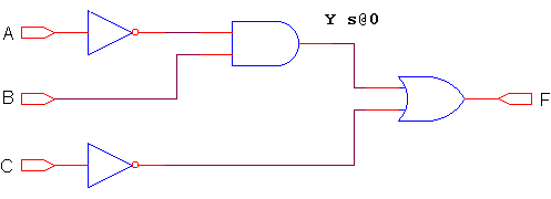
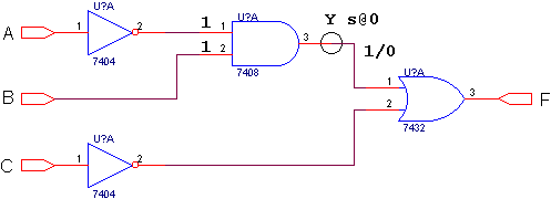
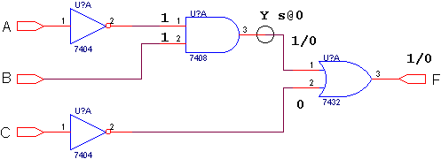
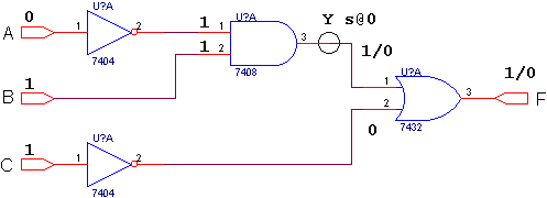
Considering the fault Y s@0 in the same circuit previously considered, figure 1 shows the result of the application of the three-step D-algorithm described:

(a) Node Y s@0.
 

(b) Fault activation (step 1).
 

(c) Fault propagation (step 2).
 

(d) Fault justification (step 3).

Figure 1: Test vector generation according to the D-algorithm.

Only the test vector (A,B,C)=(0,1,1) is able to detect the fault s@0 in node Y, since no other combination at the circuit inputs will simultaneously try to force the opposite value at the s@ node and propagate the error signal to the circuit output. It is however common that more than one vector exists to detect a given fault, such as happens if we consider the fault s@1 in this same node Y. For this case, and considering that setting one of the AND inputs to 0 will force a 0 in the node (if it is not s@1) and that C=1 guarantees propagation of the error signal, we have three vectors able to detect the fault Y s@1: (A,B,C) = { (0,0,1) | (1,0,1) | (1,1,1)}. The reader my confirm that any of these three test vectors is able to detect this fault, using the interactive schematic diagram shown in figure 2.

No Way!

Figure 2: Interactive schematic diagram for Y s@1.

An opposite situation may also take place, when there are no vectors able to detect a given fault. Figure 3 presents an interactive schematic to illustrate the case of Y s@0 (but now with a slightly different circuit with only two inputs), where it is not possible to try to force a 1 in the faulty node and at the same time to propagate the resulting error signal to the circuit output (the A input should be simultaneously 0 and 1).

Figure 3: Intereactive schematic diagram for the case of an undetectable fault.

There are however some cases where a test vector may still be found even if we momentarily come to a conflicting situation, provided that it is possible to backtrack to a previous decision point and choose a different solution. In the interactive example shown in figure 4, and when a first choice of (A,B)=(0,0) is seen to be impossible, the alternative solution of (A,B)=(1,1) leads to the required test vector.

Figure 4: Intereactive schematic diagram to illustrate backtracking.

Test vector generation in practice is done by tools that accept a description of the circuit (such as a netlist) and search for the smallest set of test vectors able to achieve maximum fault coverage.